A&H Data: Creating Mapping Layers from Historic Maps

Some of you know that I’m rather delighted by maps. I find them fascinating for many reasons, from their visual beauty to their use of the lie to impart truth, to some of their colors and onward. I think that maps are wonderful and great and superbulous even as I unhappily acknowledge that some are dastardly examples of horror.

What I’m writing about today is the process of taking a historical map (yay!) and pinning it on a contemporary street map in order to use it as a layer in programs like StoryMaps JS or ArcGIS, etc. To do that, I’m going to write about
Picking a Map from Wikimedia Commons
Wikimedia accounts and “map” markup
Warping the map image
Loading the warped map into ArcGIS Online as a layer

But! Before I get into my actual points for the day, I’m going to share one of my very favorite maps:
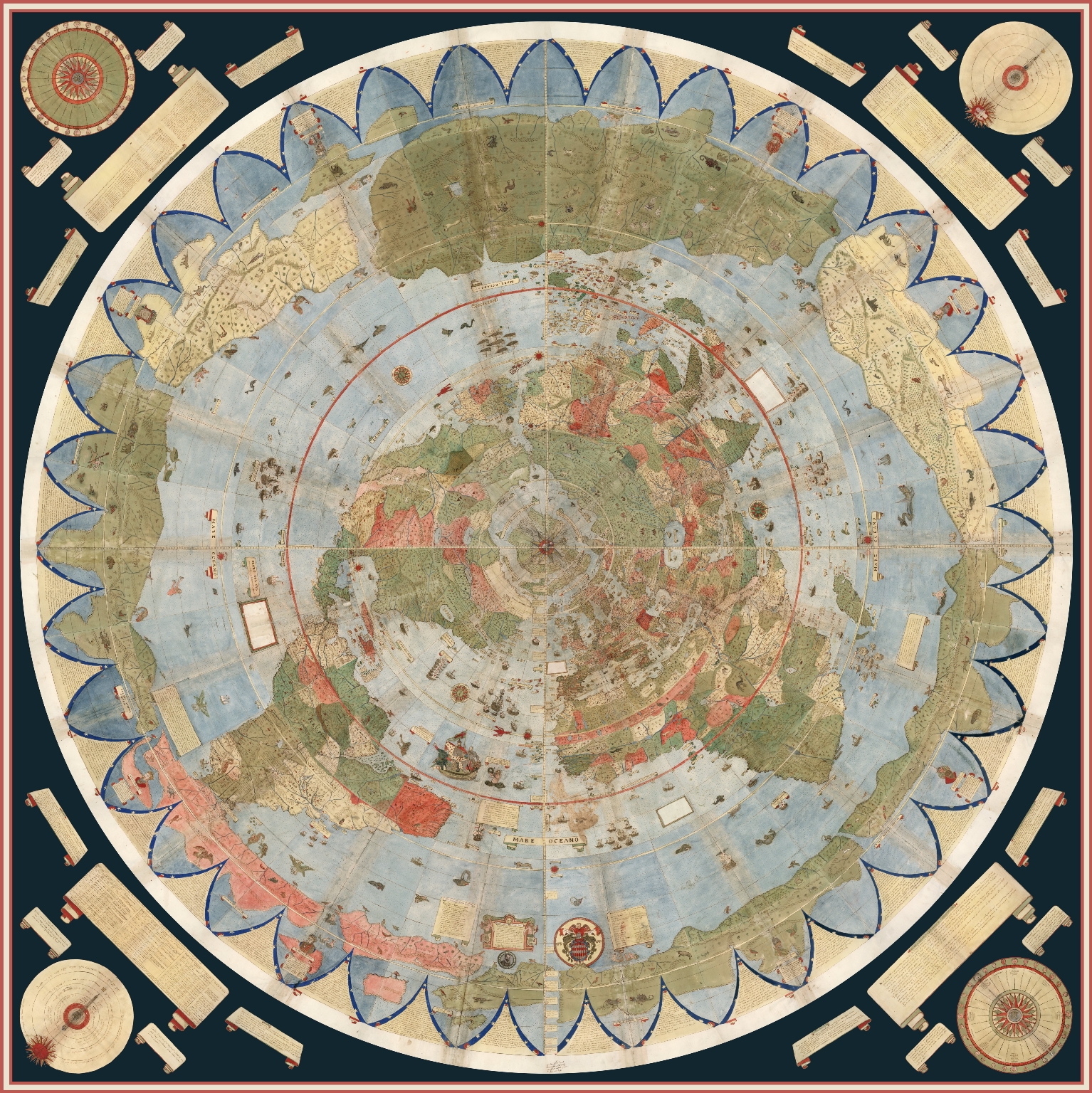
Stunning 16th century map from a northern projection with the continents spread out around the north pole in greens, blues, and reds. A black border with golds surround the circular maps.
Urbano Monte, Composite: Tavola 1-60. [Map of the World], World map, 40x51cm (Milan, Italy, 1587), David Rumsey Map Collection, http://www.davidrumsey.com.
Just look at this beauty! It’s an azimuthal projection, centered on the North Pole (more on Wikipedia), from a 16th century Italian cartographer. For a little bit about map projections and what they mean, take a look at NASA’s example Map Projections Morph. Or, take a look at the above map in a short video from David Rumsey to watch it spin, as it was designed to.

What is Map Warping

While this is in fact one of my favorite maps and l use many an excuse to talk about it, I did actually bring it up for a reason: the projection (i.e., azimuthal) is almost impossible to warp.

As stated, warping a map is when one takes a historical map and pins it across a standard, contemporary “accurate” street map following a Mercator projection, usually for the purpose of analysis or use in a GIS program, etc.

Here, for example, is the 1913 Sanborn fire insurance map layered in ArcGIS Online maps.

Image of historical Sandborn map warped across the streetmap
Screen capture of ArcGIS with rectified Sanborn map.

I’ll be writing about how I did that below. For the moment, note how the Sanborn map is a bit pinched at the bottom and the borders are tilted. The original map wasn’t aligned precisely North and the process of pinning it (warping it) against an “accurate” street map resulted in the tilting.

That was possible in part because the Sanborn map, for all that they’re quite small and specific, was oriented along a Mercator projection, permitting a rather direct rectification (i.e., warping).

In contrast, take a look at what happens in most GIS programs if one rectifies a map—including my favorite above—which doesn’t follow a Mercator projection:
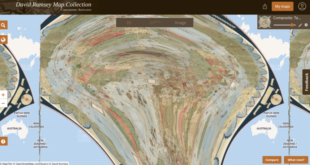
Weird looking, pulled streams of reds, greens, and blues that are swept across the top and yanked down toward the bottom.
Warped version of the Monte map against a Mercator projection in David Rumsey’s Old Maps Online connection in 2024. You can play with it in Old Maps Online.

Warping a Mercator Map

This still leaves the question: How can one warp a map to begin with?

There are several programs that you can use to “rectify” a map. Among others, many people use QGIS (open access; Windows, macOS, Linux) or ArcGIS Pro (proprietary;Windows only).

Here, I’m going to use Wikimaps Warper (for more info), which connects up with Wikimedia Commons. I haven’t seen much documentation on the agreements and I don’t know what kind of server space the Wikimedia groups are working with, but recently Wikimedia Commons made some kind of agreement with Map Warper (open access, link here) and the resulting Wikimaps Warper is (as of the writing of this post in November 2024) in beta.

I personally think that the resulting access is one of the easiest to currently use.

And on to our steps!

Picking a Map from Wikimedia Commons

To warp a map, one has to have a map. At the moment, I recommend heading over to Wikimedia Commons (https://commons.wikimedia.org/) and selecting something relevant to your work.

Because I’m planning a multi-layered project with my 1950s publisher data, I searched for (san francisco 1950 map) in the search box. Wikimedia returned dozens of Sanborn Insurance Maps. At some point (22 December 2023) a previous user (Nowakki) had uploaded the San Francisco Sanborn maps from high resolution digital surrogates from the Library of Congress.

Looking through the relevant maps, I picked Plate 0000a (link) because it captured several areas of the city and not just a single block.

When looking at material on Wikimedia, it’s a good idea to verify your source. Most of us can upload material into Wikimedia Commons and the information provided on Wikimedia is not always precisely accurate. To verify that I’m working with something legitimately useful, I looked through the metadata and checked the original source (LOC). Here, for example, the Wikimedia map claims to be from 1950 and in the LOC, the original folder says its from 1913.

Feeling good about the legality of using the Sanborn map, I was annoyed about the date. Nonetheless, I decided to go for it.

Moving forward, I checked the quality. Because of how georecification and mapping software works, I wanted as high a quality of map as I could get so that it wouldn’t blur if I zoomed in.

If there wasn’t a relevant map in Wikimedia Commons already, I could upload a map myself (and likely will later). I’ll likely talk about uploading images into Wikimedia Commons in … a couple months maybe? I have so many plans! I find process and looking at steps for getting things done so fascinating.

Wikimedia Accounts and Tags
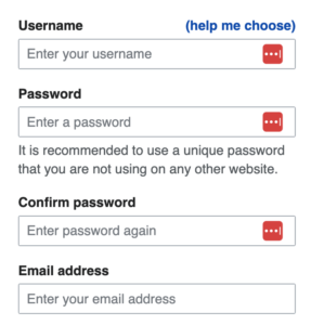
Form in whites and blacks with options for a username, password.
Signup form for the Wikimedia suite, including Wikimedia Commons and Wikimaps.

Before I can do much with my Sanborn map, I need to log in to Wikimedia Commons as a Wiki user. One can set up an account attached to one of one’s email accounts at no charge. I personally use my work email address.

Note: Wikimedia intentionally does not ask for much information about you and states that they are committed to user privacy. Their info pages (link) states that they will not share their users’ information.

I already had an account, so I logged straight in as “AccidentlyDigital” … because somehow I came up with that name when I created my account.

Once logged in, a few new options will appear on most image or text pages, offering me the opportunity to add or edit material.

Once I picked the Sanborn map, I checked

  1. Was the map already rectified?
  2. Was it tagged as a map?

If the specific map instance has already been rectified in Wikimaps, then there should be some information toward the end of the summary box that has a note about “Geotemporal data” and a linked blue bar at the bottom to “[v]iew the georeferenced map in the Wikimaps Warper.”

WikiMaps screen capture of the "Summary" with the geobox information showing the map's corner cordinants and a link to viewing it on Wikimaps.
Screen capture of “Summary” box with geocordinates from 2024.

If that doesn’t exist, then one might get a summary box that is limited to a description, links, dates, etc., and no reference to georeferencing.

In consequence, I needed to click the “edit” link next to “Summary” above the description. Wikimedia will then load the edit box for only the summary section, which will appear with all the text from the public-facing box surrounded by standard wiki-language markup.

Summary box showing a limited amount of information with purple headers to the left and information to the right on a grey background.
Screen capture of Wikimedia Commons box with limited information for an image.

All I needed to do was change the “{{Information” to “{{Map” and then hit the “Publish” button toward the bottom of the edit box to release my changes.
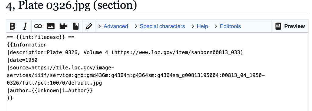
Screen capture of wikimedia commons edit screen showing what the text for updating a summary looks like.
Screen capture of Wikimedia Commons edit screen for the summary.

The updated, public-facing view will now have a blue button offering to let users “Georeference the map in Wikimaps Warper.”

Once the button appeared, I clicked that lovely, large, blue button and went off to have some excellent fun (my version thereof).
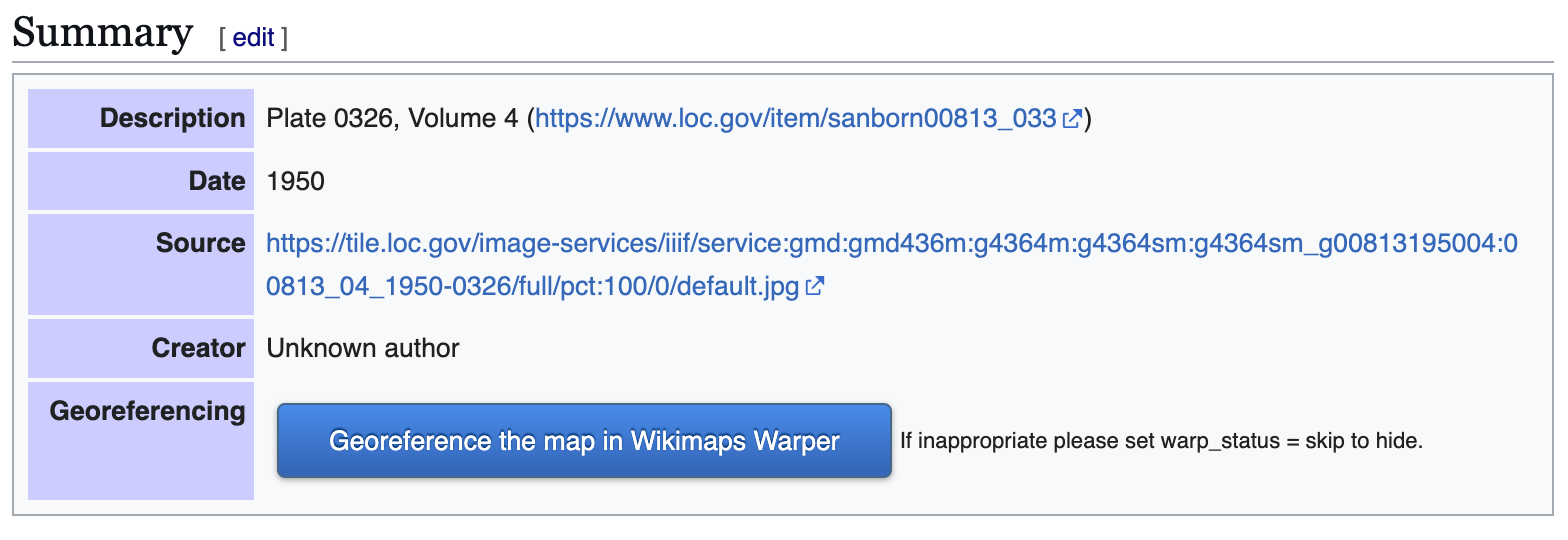
Summary box with map added as object type with blue box for options for georeferencing.
Example of Wikimedia Commons Summary box prior to georeferencing.

Warping the map

When I clicked the “Georefence” button, Wikimedia sent me away to Wikimaps Warper (https://warper.wmflabs.org/). The Wikimaps interface showed me a thumbnail of my chosen map and offered to let me “add this map.”

I, delighted beyond measure, clicked the button and then went and got some tea. Depending on how many users are in the Wikimaps servers and how big the image file for the map is, adding the file into the Wikimaps servers can take between seconds and minutes. I have little patience for uploads and almost always want more tea, so the upload time is a great tea break.

Once the map loaded (I can get back to the file through Wikimedia Commons if I leave), I got an image of my chosen map with a series of options as tabs above the map.

Most of the tabs attempt to offer options for precisely what they say. The “Show” tab offers an image of the loaded map.

Wikimaps Warper navigation tabs in beiges and white tabs showing the selected tabs.
2024 screen capture showing navigation tabs.
  • Edit allows me to edit the metadata (i.e., title, cartographer, etc.) associated with the map.
  • Rectify allows me to pin the map against a contemporary street map.
  • Crop allows me to clip off edges and borders of the map that I might not want to appear in my work.
  • Preview allows me to see where I’m at with the rectification process.
  • Export provides download options and HTML links for exporting the rectified map into other programs.
  • Trace would take me to another program with tracing options. I usually ignore the tab, but there are times when it’s wonderful.

The Sanborn map didn’t have any information I felt inclined to crop, so I clicked straight onto the “Rectify” tab and got to work.

As noted above, the process of rectification involves matching the historic map against a contemporary map. To start, one needs at least four pins matching locations on each map. Personally, I like to start with some major landmarks. For example, I started by finding Union Square and putting pins on the same location in both maps. Once I was happy with my pins’ placement on both maps, I clicked the “add control point” button below the two maps.
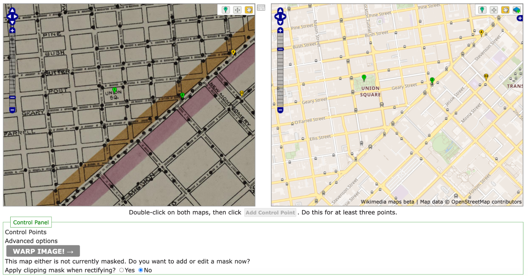
split screen showing a historic, streetmap on the left with a
Initial pins set in the historic map on the left and the OpenStreetMap on the right. note the navigation tools in the upper right corner of each panel.

Once I had four pins, I clicked the gray “warp image!” button. The four points were hardly enough and my map curled badly around my points.

To straighten out the map, I went back in and pinned the four corners of the map against the contemporary map. I also pinned several street corners because I wanted the rectified map to be as precisely aligned as possible.

All said, I ended up with more than 40 pins (i.e., control points). As I went, I warped the image every few pins in order to save it and see where the image needed alignment.
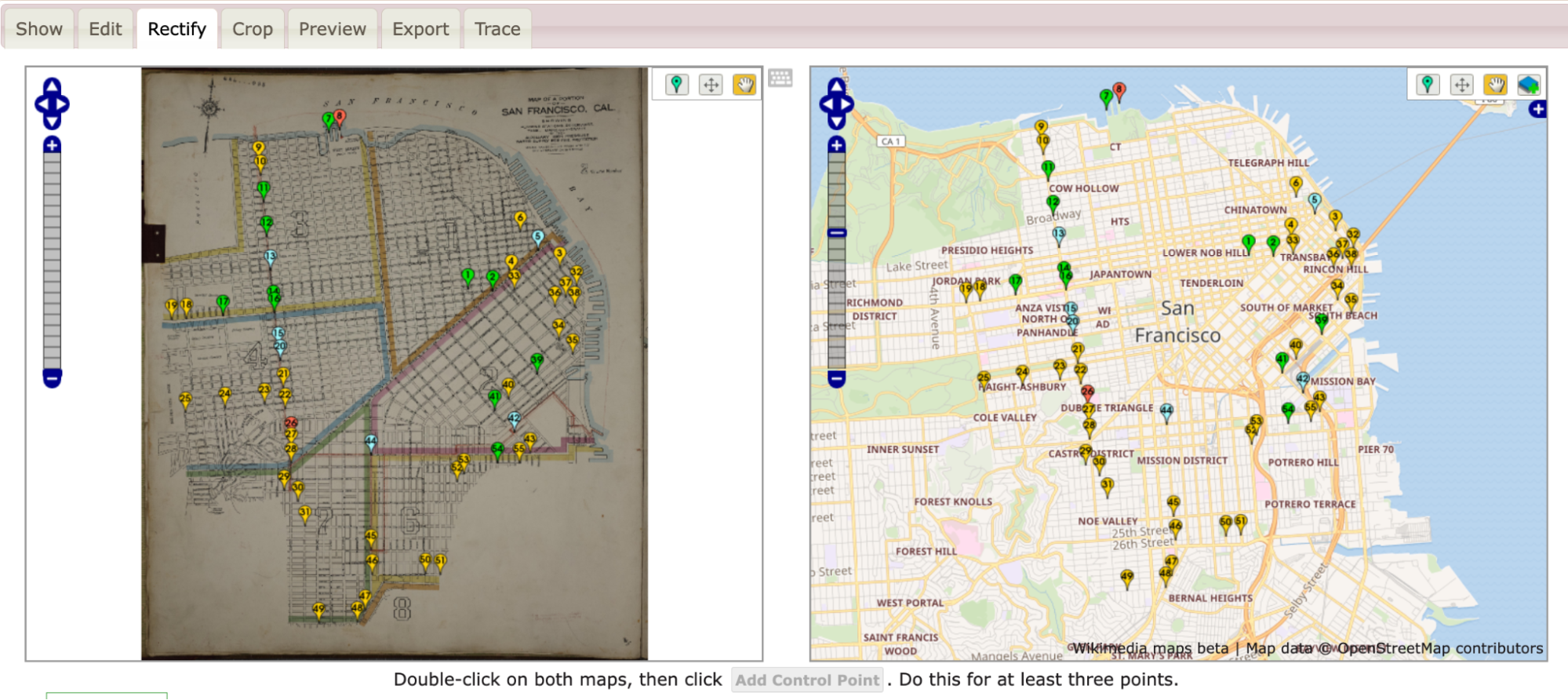
Split screen example showing dozens of aligned points in green, yellow, and red.
Screen capture of Wikimaps with example of pins for warping.

As I added control points and warped my map, the pins shifted colors between greens, yellows, and reds with the occasional blue. The colors each demonstrated where the two maps were in exact alignment and where they were being pinched and, well, warped, to match.

Loading the warped map into ArcGIS Online as a layer

Once I was happy with the Sanborn image rectified against the OpenStreetMap that Wikimaps draws in, I was ready to export my work.

In this instance, I eventfully want to have two historic maps for layers and two sets of publisher data (1910s and 1950s).

To work with multiple layers, I needed to move away from Google My Maps and toward a more complex GIS program. Because UC Berkeley has a subscription to ArcGIS Online, I headed there. If I hadn’t had access to that online program, I’d have gone to QGIS. For an access point to ArcGIS online or for more on tools and access points, head to the UC Berkeley Library Research Guide for GIS (https://guides.lib.berkeley.edu/gis/tools).

I’d already set up my ArcGIS Online (AGOL) account, so I jumped straight in at https://cal.maps.arcgis.com/ and then clicked on the “Map” button in the upper-left navigation bar.

Green and white navigation bar with map, screen, groups, content, and more
2024 Screen capture of ArcGIS Online Navigation Bar from login screen
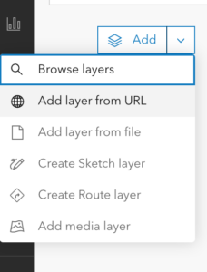
ArcGIS Online add layer list in white and blacks, offering options for layer sourcing from URL, file, sketching, route, or other media.
2024 add layer list in ArcGIS Online

On the Map screen, ArcGIS defaulted to a map of the United States in a Mercator projection. ArcGIS also had the “Layers” options opened in the left-hand tool bars.

Because I didn’t yet have any layers except for my basemap, ArcGIS’s only option in “Layers” was “Add.”

Clicking on the down arrow to the right of “Add,” I selected “Add layer from URL.”

In response, ArcGIS Online gave me a popup box with a space for a URL.

I flipped back to my Wikimaps screen and copied the “Tiles (Google/OSM scheme),” which in this case read https://warper.wmflabs.org/maps/tile/7258/{z}/{x}/{y}.png.

Flipping back to ArcGIS Online, I pasted the tile link into the URL text box and made sure that the auto-populating “Type” information about the layer was accurate. I then hit a series of next to assure ArcGIS Online that I really did want to use this map.

Warning: Because I used a link, the resulting layer is drawn from Wikimaps every time I load my ArcGIS project. That does mean that if I had a poor internet connection, the map might take a hot minute to load or fail entirely. On UC Berkeley campus, that likely won’t be too much of an issue. Elsewhere, it might be.

Once my image layer loaded, I made sure I was aligned with San Francisco, and I saved my map with a relevant title. Good practice means that I also include a map description with the citation information to the Sanborn map layer so that viewers will know where my information is coming from.
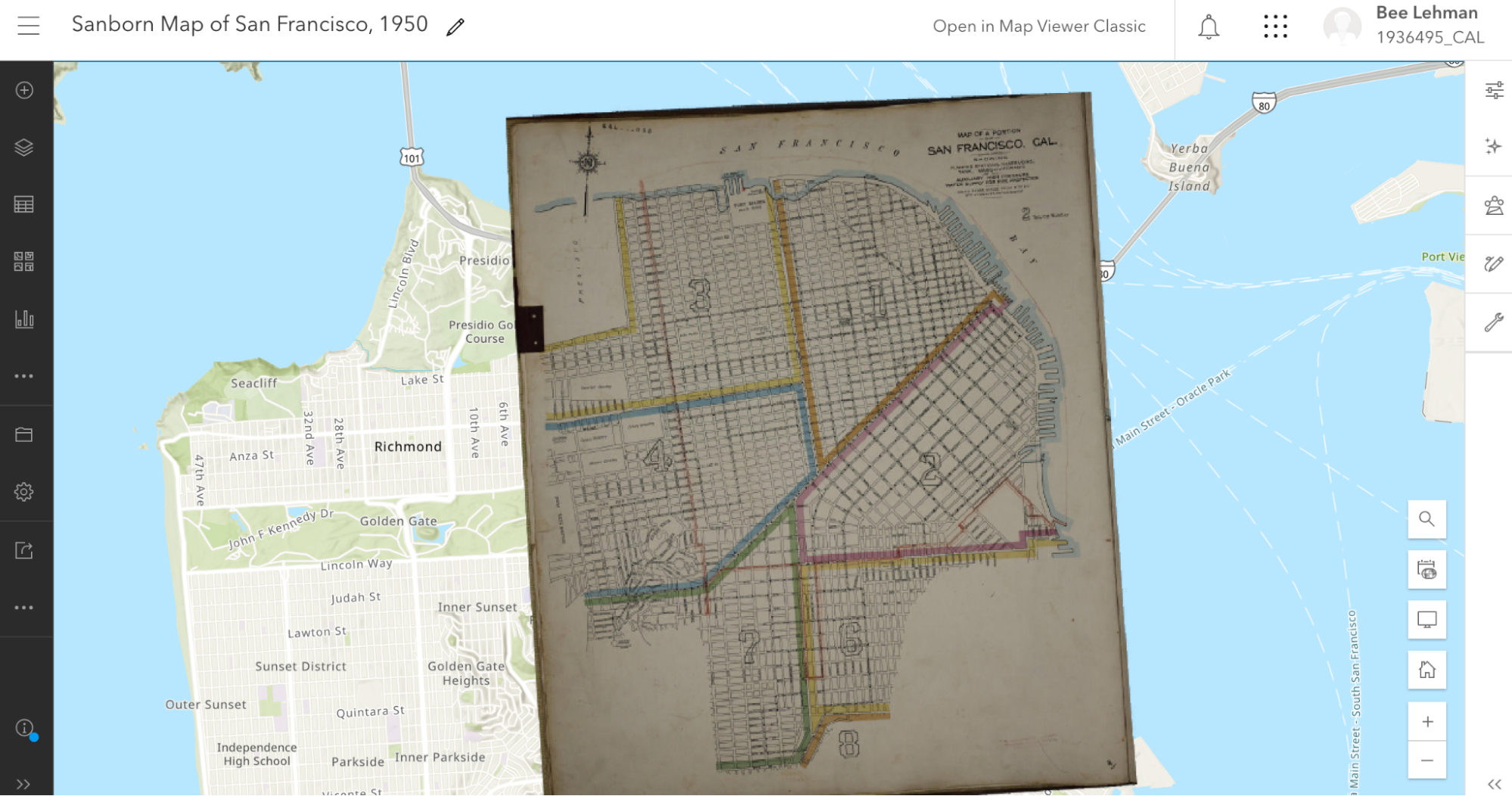
Image of historical Sandborn map warped across the streetmap
2024 Screen capture of ArcGIS maps edit screen with rectified Sanborn map.

Once I’ve saved it, I can mess with share settings and begin offering colleagues and other publics the opportunity to see the lovely, rectified Sanborn map. I can also move toward adding additional layers.

Next Time

Next post, I plan to write about how I’m going to add my lovely 1955 publisher dataset on top of a totally different, 1950 San Francisco map as a new layer. Yay!
A&H Data: Designing Visualizations in Google Maps

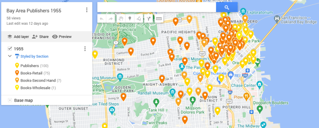
This map shows the locations of the bookstores, printers, and publishers in San Francisco in 1955 according to Polk’s Directory (SFPL link). The map highlights the quantity thereof as well as their centrality in the downtown. That number combined with location suggests that publishing was a thriving industry.

Using my 1955 publishing dataset in Google My Maps (https://www.google.com/maps/d) I have linked the directory addresses of those business categories with a contemporary street map and used different colors to highlight the different types. The contemporary street map allows people to get a sense of how the old data compares to what they know (if anything) about the modern city.

My initial Google My Map, however, was a bit hard to see because of the lack of contrast between my points as well as how they blended in with the base map. One of the things that I like to keep in mind when working with digital tools is that I can often change things. Here, I’m going to poke at and modify my

  • Base map
  • Point colors
  • Information panels
  • Sharing settings

My goal in doing so is to make the information I want to understand for my research more visible. I want, for example, to be able to easily differentiate between the 1955 publishing and printing houses versus booksellers. Here, contrasting against the above, is the map from the last post:

Image of the My Mpas backend with pins from the 1955-56 polk directory, colors indicating publishers or booksellers.
Click on the map for the last post in this series.

Quick Reminder About the Initial Map

To map data with geographic coordinates, one needs to head to a GIS program (US.gov discussion of). In part because I didn’t yet have the latitude and longitude coordinates filled in, I headed over to Google My Maps. I wrote about this last post, so I shan’t go into much detail. Briefly, those steps included:

    1. Logging into Google My Maps (https://www.google.com/maps/d/)
    2. Clicking the “Create a New Map” button
    3. Uploading the data as a CSV sheet (or attaching a Google Sheet)
    4. Naming the Map something relevant

Now that I have the map, I want to make the initial conclusions within my work from a couple weeks ago stand out. To do that, I logged back into My Maps and opened up the saved “Bay Area Publishers 1955.”

Base Map

One of the reasons that Google can provide My Maps at no direct charge is because of their advertising revenue. To create an effective visual, I want to be able to identify what information I have without losing my data among all the ads.

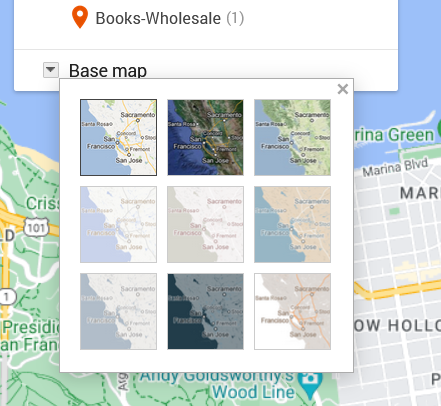
Grid of nine possible base maps for use in Google Maps. The small squares suggest different color balances and labels.
Screen capture from 2024 showing thumbnails for possible base map design.

To move in that direction, I head over to the My Map edit panel where there is a “Base map” option with a down arrow. Hitting that down arrow, I am presented with an option of nine different maps. What works for me at any given moment depends on the type of information I want my data paired with.

The default for Google Maps is a street map. That street map emphasizes business locations and roads in order to look for directions. Some of Google’s My Maps’ other options focus on geographic features, such as mountains or oceans. Because I’m interested in San Francisco publishing, I want a sense of the urban landscape and proximity. I don’t particularly need a map focused on ocean currents. What I do want is a street map with dimmer colors than Google’s standard base map so that my data layer is distinguishable from Google’s landmarks, stores, and other points of interest.

Nonetheless, when there are only nine maps available, I like to try them all. I love maps and enjoy seeing the different options, colors, and features, despite the fact that I already know these maps well.

The options that I’m actually considering are “Light Political” (option center left in the grid) “Mono City” (center of the grid) or “White Water” (bottom right). These base map options focus on that lighter-toned background I want, which allows my dataset points to stand clearly against them.

For me, “Light Political” is too pale. With white streets on light gray, the streets end up sinking into the background, losing some of the urban landscape that I’m interested in. The bright, light blue of the ocean also draws attention away from the city and toward the border, which is precisely what it wants to do as a political map.

I like “Mono City” better as it allows my points to pop against a pale background while the ocean doesn’t draw focus to the border.

Of these options, however, I’m going to go with the “White Water” street map. Here, the city is done up with various grays and oranges, warming the map in contrast to “Mono City.” The particular style also adds detail to some of the geographic landmarks, drawing attention to the city as a lived space. Consequently, even though the white water creeps me out a bit, this map gets closest to what I want in my research’s message. I also know that for this data set, I can arrange the map zoom to limit the amount of water displayed on the screen.

Point colors

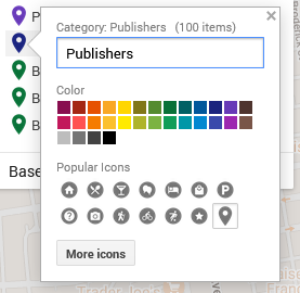
Now that I’ve got my base map, I’m on to choosing point colors. I want them to reflect my main research interests, but I’ve also got to pick within the scope of the limited options that Google provides.

Google My Map 30 color options above grid of symbols one can use for data points across map.
Color choices and symbols one can use for points as of 2024.

I head over to the Edit/Data pane in the My Maps interface. There, I can “Style” the dataset. Specifically, I can tell the GIS program to color my markers by the information in any one of my columns. I could have points all colored by year (here, 1955) or state (California), rendering them monochromatic. I could go by latitude or name and individually select a color for each point. If I did that, I’d run up against Google’s limited, 30-color palette and end up with lots of random point colors before Google defaulted to coloring the rest gray.

What I choose here is the types of business, which are listed under the column labeled “section.”

In that column, I have publishers, printers, and three different types of booksellers:

  • Printers-Book and Commercial
  • Publishers
  • Books-Retail
  • Books-Second Hand
  • Books-Wholesale

To make these stand out nicely against my base map, I chose contrasting colors. After all, using contrasting colors can be an easy way to make one bit of information stand out against another.

In this situation, my chosen base map has quite a bit of light grays and oranges. Glancing at my handy color wheel, I can see purples are opposite the oranges. Looking at the purples in Google’s options, I choose a darker color to contrast the light map. That’s one down.

For the next, I want Publishers to compliment Printers but be a clearly separate category. To meet that goal, I picked a darker purply-blue shade.

Moving to Books-Retail, I want them to stand as a separate category from the Printers and Publishers. I want them to complement my purples and still stand out against the grays and oranges. To do that, I go for one of Google’s dark greens.

Looking at the last two categories, I don’t particularly care if people can immediately differentiate the second-hand or wholesale bookstores from the retail category. Having too many colors can also be distracting. To minimize clutter of message, I’m going to make all the bookstores the same color.

Pop-ups/ Information Dock

Google My Map editing popup showing rows from dataset as a form.
Example of editable data from data sheet row.

For this dataset, the pop-ups are not overly important. What matters for my argument here is the spread. Nonetheless, I want to be aware of what people will see if they click on my different data points.

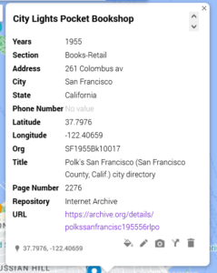
[Citylights pop-up right]

In this shot, I have an example of what other people will see. Essentially, it’s all of the columns converted to a single-entry form. I can edit these if desired and—importantly—add things like latitude and longitude.

The easiest way to drop information from the pop-up is to delete the column from the data sheet and re-import the data.

Sharing

As I finish up my map, I need to decide whether I want to keep it private (the default) or share it. Some of my maps, I keep private because they’re lists of favorite restaurants or loosely planned vacations. For example, a sibling is planning on getting married in Cadiz in Spain, and I have a map tagging places I am considering for my travel itinerary.

Toggles toward the top in blue and a close button toward the bottom for saving changes.
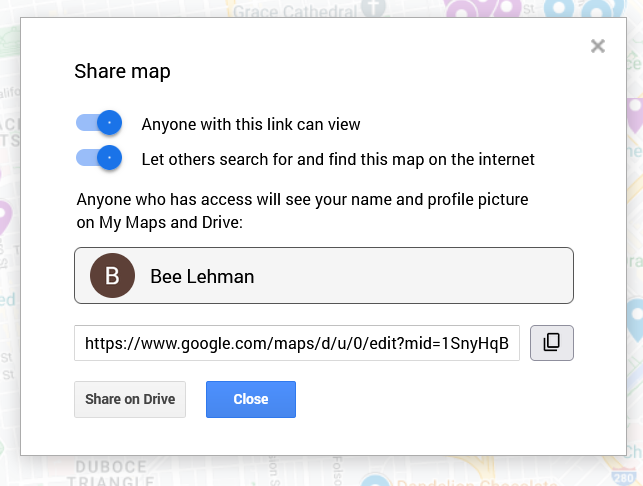
“Share map” pop up with options for making a map available.

Here, in contrast, I want friends and fellow interested parties to be able to see it and find it. To make sure that’s possible, I clicked on “Share” above my layers. On the pop-up (as figured here) I switched the toggles to allow “Anyone with this link [to] view” and “Let others search for and find this map on the internet.” The latter, in theory, will permit people searching for 1955 publishing data in San Francisco to find my beautiful, high-contrast map.

Important: This is also where I can find the link to share the published version of the map. If I pull the link from the top of my window, I’d share the editable version. Be aware, however, that the editable and public versions look a pinch different. As embedded at the top of this post, the published version will not allow the viewer to edit the material and will have the sidebar for showing my information, as opposed to the edit view’s pop-ups.

Next steps

To see how those institutions sit in the 1950s world, I am inclined to see how those plots align across a 1950s San Francisco map. To do that, I’d need to find an appropriate map and add a layer under my dataset. At this time, however, Google Maps does not allow me to add image and/or map layers. So, in two weeks I’ll write about importing image layers into Esri’s ArcGIS.


A&H Data: Bay Area Publishing and Structured Data

Last post, I promised to talk about using structured data with a dataset focused on 1950s Bay Area publishing. To get into that topic, I’m going to talk about 1) setting out with a research question as well as 2) data discovery, and 3) data organization, in order to do 4) initial mapping.

Background to my Research

When I moved to the Bay Area, I (your illustrious Literatures and Digital Humanities Librarian) started exploring UC Berkeley’s collections. I wandered through the Doe Library’s circulating collections and started talking to our Bancroft staff about the special library and archive’s foci. As expected, one of UC Berkeley’s collecting areas is California publishing, with a special emphasis on poetry.

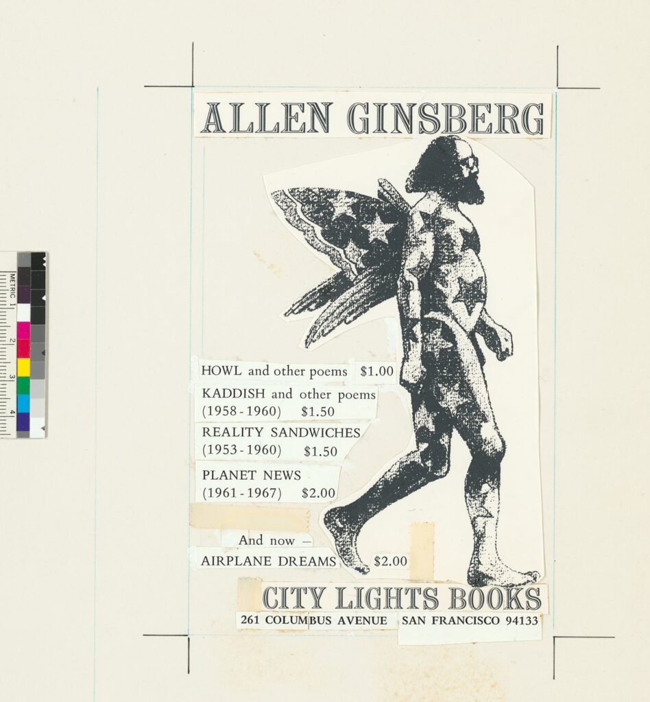
Allen Ginsberg depicted with wings in copy for a promotional piece.
Mock-up of ad for books by Allen Ginsberg, City Lights Books Records, 1953-1970, Bancroft Library.

In fact, some of Bancroft’s oft-used materials are the City Light Books collections (link to finding aids in the Online Archive of California) that include some of Allen Ginsberg’s pre-publication drafts of “Howl” and original copies of Howl and Other Poems. You may already know about that poem because you like poetry, or because you watch everything with Daniel Radcliffe in it (IMDB on the 2013 Kill your Darlings). This is, after all, the very poem that led to the seminal trial that influenced U.S. free speech and obscenity laws (often called The Howl Obscenity Trial) . The Bancroft collections have quite a bit about that trial as well as some of Ginsberg’s correspondence with Lawrence Ferlinghetti (poet, bookstore owner, and publisher) during the harrowing legal case. (You can a 2001 discussion with Ferlinghetti on the subject here.)

Research Question

Interested in learning more about Bay Area publishing in general and the period in which Ginsberg’s book was written in particular, I decided to look into the Bay Area publishing environment during the 1950s and now (2020s), starting with the early period. I wanted a better sense of the environment in general as well as public access to books, pamphlets, and other printed material. In particular, I wanted to start with the number of publishers and where they were.

Data Discovery

For a non-digital, late 19th and 20th century era, one of the easiest places to start getting a sense of mainstream businesses is to look in city directories. There was a sweet spot in an era of mass printing and industrialization in which city directories were one of the most reliable sources of this kind of information, as the directory companies were dedicated to finding as much information as possible about what was in different urban areas and where men and businesses were located. The directories, as a guide to finding business, people, and places, were organized in a clear, columned text, highly standardized and structured in order to promote usability.

Raised in an era during which city directories were still a normal thing to have at home, I already knew these fat books existed. Correspondingly, I set forth to find copies of the directories from the 1950s when “Howl” first appeared. If I hadn’t already known, I might have reached out to my librarian to get suggestions (for you, that might be me).

I knew that some of the best places to find material like city directories were usually either a city library or a historical society. I could have gone straight to the San Francisco Public Library’s website to see if they had the directories, but I decided to go to Google (i.e., a giant web index) and search for (historic san francisco city directories). That search took me straight to the SFPL’s San Francisco City Directories Online (link here).

On the site, I selected the volumes I was interested in, starting with Polk’s Directory for 1955-56. The SFPL pages shot me over to the Internet Archive and I downloaded the volumes I wanted from there.

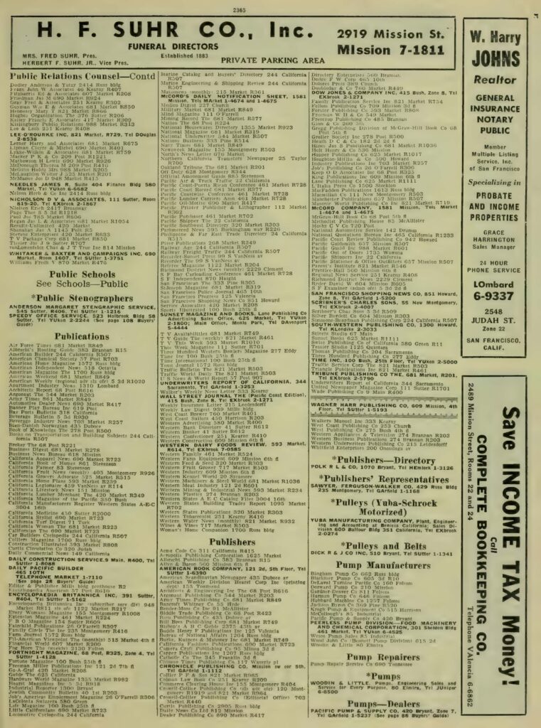
Once the directory was on my computer, I opened it and took a look through the “yellow pages” (i.e., pages with information sorted by business type) for “publishers.”

Page from a city directory with columns of company names and corresponding addresses.
Note the dense columns of text almost overlap. From R.L. Polk & Co, Polk’s San Francisco City Directory, vol. 1955–1956 (San Francisco, Calif. : R.L. Polk & Co., 1955), Internet Archive. | Public Domain.

Glancing through the listings, I noted that the records for “publishers” did not list City Light Books. Flipped back to “book sellers,” I found it. That meant that other booksellers could be publishers as well. And, regardless, those booksellers were spaces where an audience could acquire books (shocker!) and therefore relevant. Considering the issue, I also looked at the list for “printers,” in part to capture some of the self-publishing spaces.

I now had three structured lists from one directory with dozens of names. Yet, the distances within the book and inability to reorganize made them difficult to consider together. Furthermore, I couldn’t map them with the structure available in the directory. In order to do what I wanted with them (i.e., meet my research goals), I needed to transform them into a machine readable data set.

Creating a Data Set

Machine Readable

I started by doing a one-to-one copy. I took the three lists published in the directory and ran OCR across them in Adobe Acrobat Professional (UC Berkeley has a subscription; for OA access I recommend Transkribus or Tesseract), and then copied the relevant columns into a Word document.

Data Cleaning

The OCR copy of the list was a horrifying mess with misspellings, cut-off words, Ss understood as 8s, and more. Because this was a relatively small amount of data, I took the time to clean the text manually. Specifically, I corrected typos and then set up the text to work with in Excel (Google Sheets would have also worked) by:

  • creating line breaks between entries,
  • putting tabs between the name of each institution and corresponding address

Once I’d cleaned the data, I copied the text into Excel. The line breaks functioned to tell Excel where to break rows and the tabs where to understand columns. Meaning:

  • Each institution had its own row.
  • The names of the institutions and their addresses were in different columns.

Having that information in different spaces would allow me to sort the material either by address or back to its original organization by company name.

Adding Additional Information

I had, however, three different types of institutions—Booksellers, Printers, and Publishers—that I wanted to be able to keep separate. With that in mind, I added a column for EntryType (written as one word because many programs have issues with understanding column headers with spaces) and put the original directory headings into the relevant rows.

Knowing that I also wanted to map the data, I also added a column for “City” and another for “State” as the GIS (i.e., mapping) programs I planned to use wouldn’t automatically know which urban areas I meant. For these, I wrote the name of the city (i.e., “San Francisco”) and then the state (i.e., “California”) in their respective columns and autofilled the information.

Next, for record keeping purposes, I added columns for where I got the information, the page I got it from, and the URL for where I downloaded it. That information simultaneously served for me as a reminder but also as a pointer for anyone else who might want to look at the data and see the source directly.

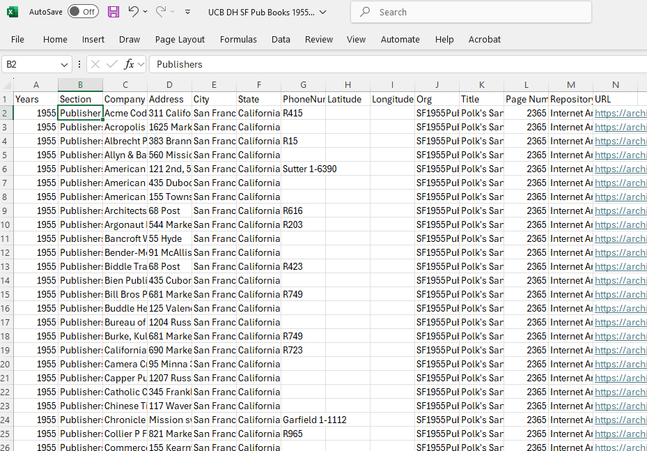
I put in a column for Org/ID for later, comparative use (I’ll talk more about this one in a further post,) and then added columns for Latitude and Longitude for eventual use.

Page from a city directory with columns of company names and corresponding addresses.
The column headers here are: Years; Section; Company; Address; City; State; PhoneNumber; Latitude; Longitude; Org; Title; PageNumber; Repository; URL. Click on the chart to see the file.

Finally, I saved my data with a filename that I could easily use to find the data again. In this case, I named it “BayAreaPublishers1955.” I made sure to save the data as an Excel file (i.e., .xmlx) and Comma Separated Value file (i.e., .csv) for use and preservation respectively. I also uploaded the file into Google Drive as a Google Sheet so you could look at it.

Initial Mapping of the Data

With that clean dataset, I headed over to Google’s My Maps (mymaps.google.com) to see if my dataset looked good and didn’t show locations in Los Angeles or other spaces. I chose Google Maps for my test because it is one of the easiest GIS programs to use

  1. because many people are already used to the Google interface
  2. the program will look up latitude and longitude based on address
  3. it’s one of the most restrictive, meaning users don’t get overwhelmed with options.

Heading to the My Maps program, I created a “new” map by clicking the “Create a new map” icon in the upper, left hand corner of the interface.

From there, I uploaded my CSV file as a layer. Take a look at the resulting map:

Image of the My Mpas backend with pins from the 1955-56 polk directory, colors indicating publishers or booksellers.
Click on the map for an interactive version. Note that I’ve set the pins to differ in column by “type.”

The visualization highlights the centrality of the 1955 San Francisco publishing world, with its concentration of publishing companies and bookstores around Mission Street. Buying books also necessitated going downtown, but once there, there was a world of information at one’s fingertips.

Add in information gleaned from scholarship and other sources about book imports, custom houses, and post offices, and one can start to think about international book trades and how San Francisco was hooked into it.

I’ll talk more about how to use Google’s My Maps in the next post in two weeks!